Intro to Control Theory Part 1: PID

This post is an intro to Control Theory, aimed at a complete beginner.

First, what is Control Theory anyways? Control Theory is the branch of engineering that deals with applying inputs to a system to get a specific output. If that sounds vague, it's because it is! The beauty of Control Theory is that it can apply to many different scenarios and systems. But that's not very useful when you're first learning, so let's look at a few specific examples of Control Theory in action:

• A self driving car: The computer applies inputs (throttle, break, wheel position, etc) to the system (the car) in order to keep in on the road and drive it to it's destination.
• A quadcopter: In fancier quadcopters, there is an onboard controller that can read from accelerometers and gyroscopes and automatically hold or go to specific positions.
• An elevator: The elevator will apply force to the carriage in order to get it to the correct floor.

For this example, we'll look at controlling an elevator. Here's what the situation looks like:

• The elevator has a position (We'll call it x). In this case, we'll say that x is measured in meters and can range from 0 to 10.
• We want the elevator to be at a specific location (We'll call goal)
• We can apply a force to the elevator. Remember, this won't cause instantaneous motion - the elevator will accelerate and decelerate. We'll call this input u.
• Gravity is always acting on the elevator - it we apply no force, it'll fall!

How do you get the elevator to go to a specific location? Let's think about writing some code. (I'm using javascript, but the concepts should be clear):

// Function to control our elevator. Returns a
// value from -1.0 to 1.0, depending on what
// force you want to apply to the elevator.
function control(x, goal) {
  // We'll need to do *something* here
}

Imagine that our control function will get called in a loop, with updated x and goal values being passed in every time it's called.

Let's try something!

function control(x, goal) {
  return 1.0;
}

Here's a simulation of that! The gray box is the elevator, and the green line is the goal. Press "Run!" to run the simulation! You can edit the code to see what happens in different situations. Press "Run!" again to restart the simulation with the new code.

Uh oh, our elevator keeps crashing into the ceiling! That's no good! We should probably take the x and goal values into account. Let's try again:

function control(x, goal) {
  if (x < goal) {
    return 1.0;
  } else if (x > goal) {
    return -1.0;
  } else {
    return 0.0;
  }
}

With this code, if the elevator is below it's goal, it goes up, and if it's higher than it's goal, it goes down! This is called "bang-bang" control.

Try it out!

This gets the elevator to the goal, but there are a few problems:

• Once it gets to it's goal, it'll still have momentum, and it'll keep going past it's goal.
• This will tend to shake around a lot at the goal position - our passengers won't be happy with this!
• In reality, the elevator will almost never be exactly at the goal. Because of this, it never ends up applying zero force, and never finishes!

How can we fix this? Think about it a bit on your own before you go on.

...

...

...

...

The simplest way to fix the problems in bang-bang control is to change the amount of force that you're applying depending on how far you are away from the goal. Mathematically, that looks like this:

\[ u = (goal - x) \times gain_{p} \]

Here's what that might look like in code:

function control(x, goal) {
  error = goal - x;
  p_gain = 0.3;
  return error * p_gain;
}

There's a few things going on here, so let's break it down:

error = goal - x;

This is an important concept in control theory - error. Error is how far you are away from your goal.

p_gain = 0.1;

This is another important concept - a gain. A gain specifies how much weight you put on a specific thing - in this case, the value is somewhat made up, as we haven't specified what the output unit is, so we don't know how much we need to multiply the error by to get a reasonable output. This is called the "P" gain because it is directly Proportional to the error.

return error * p_gain;

We multiply our error by our proportional gain to get the output force we're applying. In this case, the output is capped to the -1.0 to 1.0 range elsewhere in the code. Play around with it! Try adjusting the p_gain. And make sure that you try with the goal both above and below the elevator! Since it's being pulled down by gravity, it'll go down faster than it goes up.

This is a bit better than the bang-bang code, but it's still a long way from perfect. Here are a few problems with it:

• It still doesn't apply zero force to the elevator until it's already at it's goal. Because of this, it may still overshoot the goal.
• When the elevator is at the goal, it will apply zero force. However, gravity is still pulling the elevator down, so we really should be providing a small amount of force to resist gravity!

How do we fix this? PID!

PID stands for Proportional-Integral-Derivative control, and it solves both of the problems above. In order to understand it, you need to know a bit of calculus (but not too much, don't worry!). Feel free to skip/skim the next part if you've taken a calculus class before.

We'll need to know two definitions in order to understand PID:

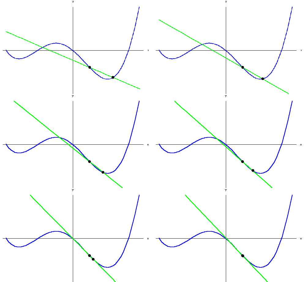
• The Derivative: The derivative is essentially the slope of a line at a specific point. This can also be thought of as how fast something is moving. For example, the derivative of position is velocity. Derivatives are often written as \(\frac{dy}{dx}\).
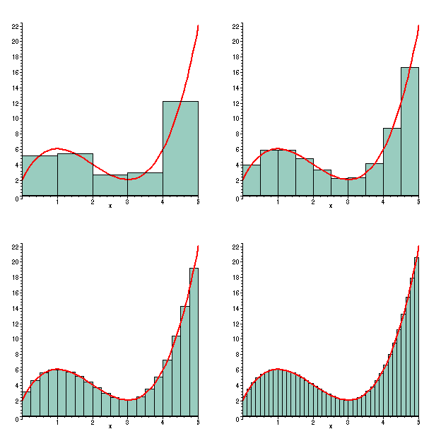
• The Integral: The integral is the area underneath a curve. This is important, because it is the reverse of the derivative. The integral is written as \(\int\).

Importantly, as the images below show, you can calculate an approximation of the integral and derivative easily.

Alright, that's enough calculus review, let's move on to the fun stuff - PID!

Our code before was just Proportional control - the P in PID - but it has two problems:

1. It overshoots the goal, because it only applies zero force once it reaches the goal!
2. It will never reach goal, because it's applying zero force, but gravity is still pulling it down.

We'll solve these one at a time:

The first problem is that we don't start slowing down until we're already past our goal, so we're going much too fast when we get there. We can solve this by applying a force to slow us down depending on how fast we're going. Recall that the derivative is how fast something's changing, so if we want our force to change depending on how fast we're going, it'll be proportional to the derivative of the error. In math terms, here's what that looks like:

\[ e = goal - x \]

\[ u = (gain_{p} \times e) - (gain_{d} \times \frac{d_{e}}{d_{t}}) \]

This is basically the same as the formula from before, but with one addition:

\[ - (gain_{d} \times \frac{d_{e}}{d_{t}}) \]

This means that we will subtract from the force that we are applying some value that is proportional to how fast the error is changing (that is, it's proportional to the derivative of the error). So how does this look in code? We can think of it as the amount that the error has changed since the last time control() was called. Here's how that looks in code:

function control(x, goal) {
  p_gain = 0.6;
  d_gain = 2.5;

  error = goal - x;
  deriv = x - this.getGlobal("last_x");

  this.setGlobal("last_x", x);

  return (error * p_gain) - (deriv * d_gain);
}

this.getGlobal() and this.setGlobal() are just an ugly way to have variables that persist across calls of the function and return zero instead of undefined. Also, notice that I've increased the p_gain. Since we now slow down when approaching the goal, we can afford to go faster on the proportional values.

As usual, play around with this code before you go on!

This looks pretty good! There's one small issue though... Try adding console.log(error) to that function somewhere - what do you see? (You'll need to open up the window to look at the results - Ctrl + Shift + K in firefox).

The error never actually reaches zero!

We'll solve the problem of never reaching the goal (called "steady state error") with the integral part of our PID loop. The way that this works is that we keep track of the total amount of error that we've had in the past. This means that as we continue to be off for a long time, we'll slowly start applying more and more force. Here's what that looks like in math:

\[ u = (gain_{p} \times e) + (gain_{i} \times \int_0^t e) - (gain_{d} \times \frac{d_{e}}{d_{t}}) \]

Essentially, what we'll do in code is make a variable called integral, and every time control() is called, we add the current error to this value. Then, we add to our output integral * i_gain.

Here's the code to actually do that:

function control(x, goal) {
  p_gain = 0.4;
  d_gain = 6.5;
  i_gain = 0.001

  error = goal - x;
  deriv = x - this.getGlobal("last_x");
  integral = this.getGlobal("integral") + error;

  this.setGlobal("last_x", x);
  this.setGlobal("integral", integral);

  return (error * p_gain) + (integral * i_gain) - (deriv * d_gain);
}

And here's the interactive version:

(Again, I've changed some of the gains besides I to compensate for the addition of the I term. Changing the PID gains is called tuning, and it's what you'll spend most of your time doing when you implement PID!)

This makes it reach zero, but it also introduces a new problem - once we are at zero, the integral term will still push us in the same direction that we are going! This is called "integral windup," and it's a common problem when choosing the gains for a PID loop. There are a few ways to deal with this, but we aren't going to go into them in this post.

Conclusion

In general, PID controllers tend to be a good way to control many types of systems, from physical systems like this elevator or a self driving car, to chemical systems! There are many more powerful techniques than PID available (and many ways to improve upon PID), but PID is a great introduction to control theory, and a good tool to have available.

That's all for now! I hope that you found this helpful, and if you liked it, check out my index of control theory posts!